
The Cobb-Douglas production function estimates how much output a plant, a firm or a whole economy gets from two inputs, capital and labor, and how much of the credit belongs to each. It is written Q = A · Kα · Lβ. Nearly everything useful about it sits in the two exponents: each one is an output elasticity, both can be estimated directly from data with a log-linear regression, and their sum tells you what happens to output when the entire operation is scaled up.
One correction worth making at the outset, because most short explanations get it wrong: α + β = 1 is not part of the definition. Cobb and Douglas imposed that restriction in their 1928 paper and relaxed it in later work. Leaving the exponents free is what lets the function measure increasing and decreasing returns to scale, which is most of what it is used for.
What is the Cobb-Douglas production function?
It is a model of how inputs turn into output. Two inputs are standard, capital (K) and labor (L), and a scale factor A carries everything else that affects productivity: technology, process design, management quality and workforce skill.
Charles Cobb, a mathematician, and Paul Douglas, an economist, published it in A Theory of Production in the American Economic Review in March 1928. Douglas had noticed that the split of US national income between capital and labor stayed remarkably stable across decades, and asked Cobb for a functional form that would reproduce that stability. The result is the function that still carries both their names.
The shape of the formula matters. Output is not capital plus labor, it is capital and labor multiplied together, each raised to a power. That has a concrete consequence: neither input can be zero. A plant full of machines with nobody to run them produces nothing, and so does a workforce with no equipment.
Cobb Douglas production function formula
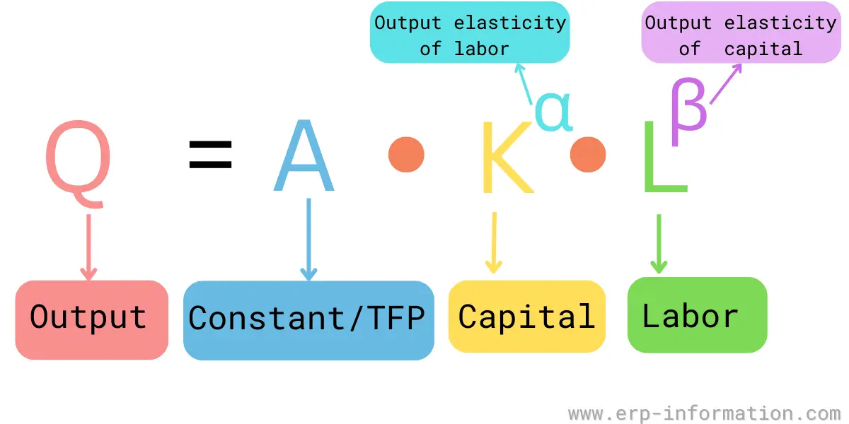
The two-input form is:
Q = A · Kα · Lβ
| Symbol | Meaning | How to read it |
|---|---|---|
| Q | Total output | Units produced, or the real value of output |
| A | Total factor productivity (TFP) | The scale factor. Everything raising output that is not a countable unit of capital or labor |
| K | Capital input | Plant, machinery, tooling and equipment |
| L | Labor input | Usually labor-hours, sometimes headcount |
| α | Output elasticity of capital | A 1% rise in K raises Q by about α% |
| β | Output elasticity of labor | A 1% rise in L raises Q by about β% |
Both exponents normally fall between 0 and 1. The exponent sits on the input it belongs to: α is attached to K, so it is capital’s elasticity, and β is attached to L.
Does α + β have to equal 1?
No, and this is the single most common error made about the function.
Cobb and Douglas did constrain the exponents to sum to 1 in the 1928 paper, and the choice was deliberate. The restriction forces constant returns to scale, and under perfect competition it makes the payments to capital and labor exactly exhaust output, which was the property Douglas wanted to test. It also made the arithmetic tractable in 1928. Later work in the 1940s relaxed it, and modern practice estimates both exponents freely.
Writing α + β = 1 into the definition quietly throws away the measurement most people came for. Returns to scale is that sum, so fixing it at 1 makes it impossible to ever detect anything else.
Cobb Douglas production function example
Take a plant with a TFP factor of 1.2, capital of 400 (thousands of dollars of plant and equipment), 900 labor-hours a week, α = 0.3 and β = 0.7:
| Step | Calculation | Result |
|---|---|---|
| Capital term | 4000.3 | 6.034 |
| Labor term | 9000.7 | 116.942 |
| Multiply through | 1.2 × 6.034 × 116.942 | 847 units per week |
The two fractional powers are the whole calculation, and they need the xy key on a calculator rather than repeated multiplication. Change any single input and the others keep their exponents, which is what makes the function convenient to work with.
Returns to scale, demonstrated
Scale both inputs by the same factor and the algebra collapses neatly. Doubling capital and labor gives:
Q(2K, 2L) = A(2K)α(2L)β = 2α+β · A Kα Lβ = 2α+β · Q
Output does not scale by 2. It scales by 2 raised to the sum of the exponents. Holding A, K, L and α fixed and varying only β shows all three regimes:
| α | β | α + β | Q at K=400, L=900 | Q at K=800, L=1800 | Output multiple | Returns to scale |
|---|---|---|---|---|---|---|
| 0.3 | 0.6 | 0.9 | 429 | 800 | 1.87 | Decreasing |
| 0.3 | 0.7 | 1.0 | 847 | 1,694 | 2.00 | Constant |
| 0.3 | 0.8 | 1.1 | 1,672 | 3,584 | 2.14 | Increasing |
The multiples are exactly 20.9 = 1.87, 21.0 = 2.00 and 21.1 = 2.14. In practical terms, doubling a plant that runs at decreasing returns buys 87% more output, not 100%, and the capital budget has to be justified against that number rather than against a doubling that will not happen.
What the exponents actually mean
Output elasticity
Raise labor by 10%, from 900 to 990 hours, and hold capital at 400. Output rises from 847 to 905, a gain of 6.9%. With β = 0.7 the elasticity predicted 7%. The small gap is expected rather than an error: an elasticity is exact only for very small changes, and 10% is not small. Most textbook statements skip that caveat, which is why hand-checked examples rarely land on the round number.
Marginal product and diminishing returns
Differentiating the function gives two compact results:
MPK = α · Q / K MPL = β · Q / L
At the base case, MPL = 0.7 × 847 / 900 = 0.659 units per extra labor-hour, and MPK = 0.3 × 847 / 400 = 0.635 units per extra unit of capital. That is easy to verify: adding a single labor-hour, from 900 to 901, moves output from 846.78 to 847.43, a gain of 0.66 units.
Because both exponents are below 1, each marginal product falls as its own input grows. Diminishing marginal returns is built into the functional form rather than bolted on as a separate assumption. The ratio MPL / MPK = (β / α) × (K / L) is the marginal rate of technical substitution: how much capital can be given up for one more unit of labor while output stays fixed.
How α and β are estimated
Take logs of both sides and the function becomes linear:
ln Q = ln A + α ln K + β ln L
That is an ordinary regression. Regress log output on log capital and log labor, and the two slope coefficients are α and β while the intercept is ln A. This is the practical reason the function dominates empirical work: it is non-linear in the variables but linear in its parameters, so ordinary least squares estimates it directly. Anything described as assuming a straight-line relationship between inputs and output has the model backwards.
Under perfect competition with constant returns, the exponents also equal the income shares. Cobb and Douglas estimated a labor exponent of 0.75 on US manufacturing data for 1899 to 1922, giving P = 1.01 · L0.75 · C0.25. That 0.75 was close to labor’s observed share of manufacturing income at the time, and the match is what made the result persuasive.
Where the Cobb-Douglas function is used
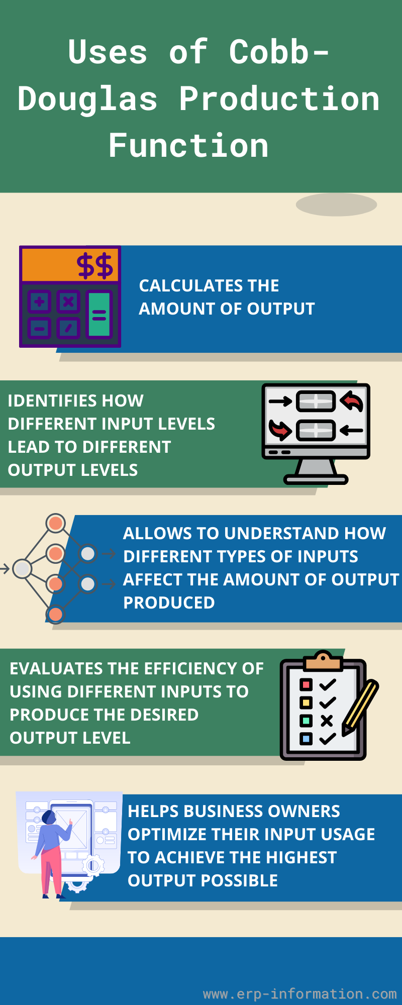
In macroeconomics it is the backbone of the Solow growth model and of growth accounting. In operations and ERP work it shows up more narrowly:
- Productivity measurement. A is total factor productivity. Fitting the function across periods separates output growth that came from adding inputs from growth that came from working better, which is the distinction a headline output number hides. Our total factor productivity growth rate calculator works the same residual.
- Scaling and capacity decisions. The sum α + β answers whether a second identical line will really double output, which is the question underneath most capacity planning business cases.
- Automation trade-offs. The marginal rate of technical substitution puts a number on how much labor a given amount of capital can replace at constant output.
- Longer-horizon planning. Because it needs only two aggregate inputs, it is usable at the level where aggregate planning and production planning actually operate, rather than requiring a full routing and bill of materials.
Limitations and criticism
The function is popular partly because it is convenient, and the convenience has costs worth stating plainly.
- It forces an elasticity of substitution of exactly 1. Whatever the real trade-off between capital and labor, Cobb-Douglas assumes a 1% change in their price ratio shifts the input ratio by 1%. No choice of α and β can change that. The CES and translog forms exist precisely to relax it, and Cobb-Douglas is the special case of CES where that elasticity equals 1.
- A good fit is weak evidence. Anwar Shaikh showed in 1974 that data points arranged to spell the word HUMBUG still fit a Cobb-Douglas function with a very high R2. His point was that any data satisfying a national accounting identity with roughly constant factor shares will fit, whether or not it describes production at all (Laws of Production and Laws of Algebra: The Humbug Production Function, Review of Economics and Statistics, 56(1), 1974, pages 115 to 120).
- Constant factor shares no longer hold. The stable labor share that motivated Douglas has been falling across industrialized economies for decades, which undercuts the empirical regularity the function was built to capture.
- Aggregate capital is contested. The Cambridge capital controversy questioned whether heterogeneous machines of different vintages can be added into a single number K at all.
- A absorbs everything unmeasured. Utilization, management quality, measurement error and any omitted input all land in the residual, so a rise in A is a prompt to investigate rather than a finding.
None of this makes the function useless. It makes it a disciplined first approximation whose assumptions should be stated rather than a law of production.
FAQs
What is the production function?
A production function is a mathematical statement of the relationship between the output a firm produces and the factors of production it uses. The most common factors are labor, capital and land.
It is used to work out total output at different levels of input use, and to identify the combination of inputs that produces a given output at least cost.
What is Leontief’s production function?
The Leontief production function assumes inputs must be used in fixed proportions, so output is set by whichever input is scarcest: Q = min(K / a, L / b).
It suits situations where inputs are not substitutable, such as one operator required per machine. Its elasticity of substitution is zero, the opposite extreme from perfect substitutes.
What is the perfect substitutes production function?
The perfect substitutes production function is the linear form Q = aK + bL, in which one input can replace the other at a fixed rate that never changes, so its isoquants are straight lines and its elasticity of substitution is infinite.
Perfect substitutes and Leontief are the two extremes of substitutability. Cobb-Douglas sits between them, with an elasticity of substitution of exactly 1.
Does alpha plus beta have to equal 1 in the Cobb-Douglas function?
No. Cobb and Douglas imposed that restriction in their 1928 paper to force constant returns to scale, and it was relaxed in later work.
The sum of the exponents is what measures returns to scale: above 1 is increasing returns, exactly 1 is constant, and below 1 is decreasing. Fixing the sum at 1 by definition makes that measurement impossible.
How do you calculate the Cobb-Douglas production function?
Raise capital to the power alpha, raise labor to the power beta, then multiply the two results together and by the productivity factor A.
For A = 1.2, K = 400, L = 900, alpha = 0.3 and beta = 0.7: 400^0.3 = 6.034 and 900^0.7 = 116.942, so Q = 1.2 x 6.034 x 116.942 = about 847 units.
Conclusion
The Cobb-Douglas function earns its place because two numbers carry a great deal of information. Each exponent is an output elasticity, and their sum is returns to scale. Being precise about that second point is what separates a useful model from a decorative one, because writing α + β = 1 into the definition discards the measurement most people opened the page to find.
Estimate the exponents from your own data rather than assuming them, treat a high R2 as a starting point rather than proof, and remember that everything you did not measure is sitting inside A.