
Part period balancing (PPB) is an MRP lot-sizing rule that keeps adding future periods’ requirements to an order until the cost of holding the extra stock roughly matches the cost of placing one order. J. J. DeMatteis published it in the IBM Systems Journal in 1968, and SAP still ships it as lot-sizing procedure SP.
The short version: divide the cost of one order by the cost of holding one unit for one period. That is the economic part period (EPP). Then grow each order one period at a time, counting units × periods held, and stop at the lot whose count is closest to the EPP. SAP’s version stops before the count would exceed it, and in our test that small change made it markedly cheaper.
This page works PPB through two full examples, shows why the textbook rule and SAP’s rule give different answers on the same data, and reports a test of 24,000 random plans comparing both with the cheapest plan possible.
What is Part Period Balancing?
Part period balancing (PPB) is a lot-size technique using look ahead and look back functions to consider additional periods in modifying an initial calculation based on the least total cost.
In plain terms: every order has a fixed cost (raising a purchase order, or setting up a machine), and every unit bought early has to be stored. Ordering more periods at once saves order costs and adds storage costs. PPB looks for the point where the two balance, because that is where the classic economic order quantity says total cost is lowest.
It works inside material requirements planning (MRP), the planning module of enterprise resource planning (ERP) systems. MRP first works out the net requirement for each period: what is needed after stock on hand and orders already placed. A lot-sizing rule then decides how those requirements are grouped into orders. PPB is one of the rules that groups them by cost.
The method was published by J. J. DeMatteis in the IBM Systems Journal in 1968. By 1983 Urban Wemmerlöv, writing in the Journal of Operations Management, called it “the most commonly used dynamic lot-sizing procedure in practice”. The look-ahead and look-back tests in the definition above are what separate PPB from the simpler least total cost rule: they were added to improve its cost by “marginally adjusting each tentative lot-size”, in Wemmerlöv’s words.
The formula: economic part period (EPP)
EPP = order (setup) cost / holding cost per unit per period
A part-period is one unit held in stock for one period. 100 units held for two weeks are 200 part-periods. The EPP is the number of part-periods whose holding cost equals one order. With an order cost of $90 and a holding cost of $0.40 per unit per week, the EPP is 90 / 0.40 = 225 part-periods: 225 units held one week, or 75 units held three weeks, cost the same $90 as placing an order.
Lot Size
A lot size is the quantity one planned order covers. Larger lots mean fewer orders and more stock on the shelf; smaller lots the reverse. Some lot sizes are set by things outside that trade-off: a machine’s batch size, a supplier’s pack size or minimum, or a customer order that must ship complete. Part period balancing is one of the rules that sets the lot from costs alone, trading order cost against holding cost to keep inventory levels down without placing an order every period.

The chart groups lot-sizing rules by what they hold fixed: a time period, a quantity, or neither. PPB sits in the third group because both the quantity and the interval can change from one order to the next.
Part Period Balancing Heuristic Method
PPB is a heuristic: a rule of thumb that is usually close to the cheapest plan but does not guarantee it. The steps:
- Calculate the EPP: order cost divided by holding cost per unit per period.
- Start a lot at the first period with a net requirement.
- Add the next period’s requirement and count its part-periods: the quantity times the number of periods it waits in stock.
- Keep adding periods while the running total moves closer to the EPP. Stop at the lot whose total is closest to it.
- Start the next lot at the next period that still has a net requirement, and repeat.
Worked example 1: ten weeks of MRP requirements
These are the same requirements we use in our period order quantity guide, so you can compare the two rules. A purchased part has 150 units on hand, an order cost of $90 and a holding cost of $0.40 per unit per week. Gross requirements for weeks 1 to 10 are 120, 0, 200, 80, 0, 160, 260, 0, 250 and 90. Opening stock covers week 1 and leaves 30 units, so the net requirements start with 170 in week 3. The EPP is 225.
| Lot | Part-periods | Holding | Decision |
|---|---|---|---|
| Weeks 3 to 4 | 80 | $32 | Both rules take it |
| Weeks 3 to 6 | 560 | $224 | Too far: both stop |
| Weeks 6 to 7 | 260 | $104 | Textbook takes it; SAP stops |
| Weeks 7 to 9 | 500 | $200 | SAP stops |
| Weeks 9 to 10 | 90 | $36 | Both rules take it |
The first lot covers weeks 3 and 4 (170 + 80 = 250 units). Holding week 4’s 80 units for one week is 80 part-periods, nearer to 225 than the 0 of a one-week lot, while stretching to week 6 jumps to 560. The last lot covers weeks 9 and 10 (340 units) for the same reason.
Week 7 is where the two versions part. Folding week 7’s 260 units into the week 6 order adds 260 part-periods. The textbook rule takes it, because 260 is only 35 away from 225. SAP’s rule refuses, because 260 is more than 225, and orders week 7 separately.
| Version | Orders | Total cost | Above best |
|---|---|---|---|
| Textbook PPB (closest) | 250, 420, 340 | $466.00 | 3.1% |
| SAP PPB (do not exceed) | 250, 160, 260, 340 | $452.00 | 0% |
SAP’s plan is the cheapest possible here: it matches the Wagner-Whitin optimum. The textbook plan pays $104 to hold 260 units for a week in order to save one $90 order, and the $14 difference is the whole gap. Both totals include the same $24 for carrying the opening stock through weeks 1 and 2.
Worked example 2: SAP’s own example
SAP’s documentation explains its procedures with one example: an item priced at 20, lot-size-independent costs (the cost of one order or setup) of 100, a storage cost percentage of 10% a year, and 1,000 pieces needed every week. Most of SAP’s pages show the money in euros; the figures work the same in any currency.

Storage cost = Requirement * Price * Storage cost % * Time in Storage / 365
Requirement Table:

Calculations for Storage Cost:
Storage Cost = (1000 * 20 * 0.1 * 7 (in days)) / 365 = 38.36
That is the cost of holding the 8 January requirement for 7 days so it can arrive with the 1 January lot. Holding the 15 January requirement for 14 days adds 76.71, so a 3,000-piece lot carries 38.36 + 76.71 = 115.07 of storage. The order is placed for 1 January and covers 1 and 8 January: 2,000 pieces. Adding the 15 January requirement would push total storage to 115.07, more than the 100 an order costs, so SAP’s rule stops at 2,000.
SAP runs its other optimum procedures on the same example in its help pages, and they do not agree:
| Procedure | First lot | Plan for 4 weeks |
|---|---|---|
| SAP part period balancing (SP) | 2,000 | $276.71 |
| SAP sliding economic lot size (WI) | 2,000 | $276.71 |
| SAP dynamic planning calculation (DY) | 3,000 | $315.07 |
| SAP Groff reorder procedure (GR) | 1,000 | $400.00 if repeated |
| Textbook PPB (closest to the EPP) | 3,000 | $315.07 |
The first-lot answers for SP, WI, DY and GR are SAP’s own. The 4-week costs and the textbook PPB answer are our calculations: two lots of 2,000 cost 2 × (100 + 38.36) = 276.71, the cheapest plan for these four weeks. The textbook rule picks 3,000 because 115.07 is closer to 100 than 38.36 is, then needs a separate order for week 4.
Evaluate storage cost using our Storage costs of inventory online calculator
Why Part Period Balancing?
PPB earns its place when requirements are uneven, which is normal for components planned by MRP. Unlike a fixed economic order quantity, it orders whole periods of demand, so no remnants are left between orders. Unlike lot-for-lot, it groups small requirements so you are not paying for an order every period.
- It adapts to the actual pattern. Each lot is sized from the requirements in front of it, not from an average, which is where period order quantity loses money.
- It needs only two cost inputs: the cost of an order and the cost of holding a unit for a period.
- You can work it by hand and explain every lot to a buyer or a supplier.
- It is built into SAP as procedure SP, so no custom logic is needed there.
Its weakness is in the stopping rule. “Closest to the EPP” treats overshooting and undershooting alike, but the costs are not alike: going over means paying more to hold stock than an order would have cost. Wemmerlöv noted “a fundamental flaw” in the model that “leads to poor performance under certain conditions”. Our test below measures how much that costs.
Textbook PPB or SAP’s version: which is cheaper?
We ran both versions of PPB, five other rules and the Wagner-Whitin optimum over 24,000 randomly generated 24-week plans, the same test as in our period order quantity guide.
| Rule | Steady | Variable | Lumpy |
|---|---|---|---|
| SAP PPB (do not exceed) | 0.9% | 3.6% | 2.8% |
| Silver-Meal | 1.1% | 1.9% | 2.7% |
| Textbook PPB (closest) | 8.6% | 10.2% | 9.7% |
| SAP dynamic planning (DY) | 11.6% | 7.8% | 3.5% |
| Least unit cost (SAP WI) | 1.3% | 16.9% | 11.8% |
| Period order quantity | 0.9% | 8.9% | 7.3% |
| Lot-for-lot | 62.1% | 75.2% | 33.5% |
| Fixed EOQ | 34.2% | 43.4% | 49.9% |
Each figure is the average cost above the cheapest possible plan. Steady demand has a standard deviation of 20% of its average, variable demand 60%, and lumpy demand has no requirement at all in 40% of weeks.
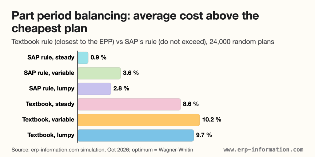
- SAP’s “do not exceed” rule beat the textbook “closest” rule in all 12 combinations of demand pattern and cost ratio we tested, cutting the average gap from 8.6% to 10.2% down to 0.9% to 3.6%.
- The textbook rule was worst when orders are cheap. With steady demand and an EOQ of about one period, it averaged 21.6% above the minimum, because it kept adding a period whenever that landed slightly nearer the EPP, even though the extra holding cost more than an order.
- Not every SAP procedure is safe everywhere. Dynamic planning (DY) averaged 28.1% above the minimum on steady demand when the EOQ covered four periods, and least unit cost (WI) 16.9% on variable demand.
How the test was run (9 October 2026): 2,000 plans for each of 3 demand patterns and 4 cost ratios, chosen so the EOQ covers 1, 2, 3 or 4 periods. Average demand 100 units a period, holding cost charged on ending stock, no opening stock, demand known for the whole 24 weeks. Our code reproduces SAP’s published answers for SP, WI and DY on SAP’s example, and its Wagner-Whitin solver matched a brute-force search on 300 small test cases. A second run with a different random seed moved no figure by more than 0.3 points. The look-ahead and look-back tests were not modelled, because published versions of them differ. The test leaves out forecast error, capacity limits and minimum order quantities.
Heuristic Methods Alternative to PPB
Apart from Part Period Balancing, there are various other methods to determine the Lot Size.

| Technique | How each order is sized |
|---|---|
| Fixed order quantity (FOQ) | A set quantity, often a pack size or supplier minimum |
| Lot-for-lot (L4L) | Exactly one period’s net requirement |
| Economic order quantity (EOQ) | A set quantity that balances order and holding cost for steady demand |
| Silver-Meal | Adds periods while the cost per period keeps falling |
| Least unit cost (LUC) | Adds periods while the cost per unit keeps falling |
| Periods of supply (POS) | The net requirements of a number of periods the planner chooses |
| Period order quantity (POQ) | The net requirements of EOQ ÷ average demand periods |
| Least total cost (LTC) | The same balance test as PPB, without the look-ahead and look-back tests |
| Wagner-Whitin | Solves for the cheapest plan over the whole horizon |
Evaluate Fixed Order Quantity using our Online Fixed Order Quantity Calculator
Evaluate Economic Order Quantity using our Online Economic Order Quantity Calculator With Graph (EOQ Calculator)
Part period balancing in ERP systems
SAP S/4HANA offers PPB as optimum lot-sizing procedure SP. In the material master (MRP 1 view), enter SP in the MRP Lot Size field along with the lot-size-independent costs and a storage costs indicator. SAP’s help describes it as grouping consecutive requirements “until the total of the storage costs is the same as the lot-size-independent costs”, and its example shows the rule never letting storage exceed that cost. SAP’s other optimum procedures are WI (sliding economic lot size), DY (dynamic planning calculation) and GR (Groff).
The other three systems we checked do not list a part period balancing option in their documentation. Oracle NetSuite offers lot for lot, fixed lot size, fixed lot multiple, minimum order quantity and periods of supply. Microsoft Dynamics 365 Business Central offers the Fixed Reorder Qty., Maximum Qty., Order and Lot-for-Lot reordering policies. Dynamics 365 Supply Chain Management offers coverage codes such as Per requirement, Per period and Min/Max. In those systems, PPB has to be calculated outside and entered as a fixed quantity or period.
If lot-sizing rules matter to your planners, put them on your ERP requirements list before you shortlist vendors, and ask each one to run a sample of your own requirements through them.
FAQs
What is part period balancing in simple terms?
It is a lot-sizing rule that keeps adding the next periods’ requirements to an order until the cost of holding the extra stock roughly equals the cost of placing one order. The balance point is the economic part period: the order cost divided by the cost of holding one unit for one period.
How do you calculate the economic part period?
Divide the cost of placing one order by the cost of holding one unit for one period. With an order cost of $90 and a holding cost of $0.40 per unit per week, the economic part period is 225 part-periods, which is 225 units held one week or 75 units held three weeks.
What is the difference between part period balancing and least total cost?
Both use the same balance test between holding cost and order cost. Urban Wemmerlöv’s 1983 study describes the look-ahead and look-back tests, which marginally adjust each tentative lot size, as the feature that distinguishes part period balancing from least total cost.
Does SAP use part period balancing?
Yes. SAP S/4HANA offers it as optimum lot-sizing procedure SP, set in the MRP Lot Size field of the material master together with the lot-size-independent costs and a storage costs indicator. SAP groups requirements until the total storage costs would exceed the lot-size-independent costs.
Is part period balancing optimal?
No. It is a heuristic. In our test of 24,000 random plans, the textbook rule averaged 9% to 10% above the cheapest plan on uneven demand and SAP’s version 3% to 4%. The Wagner-Whitin method finds the true minimum when demand is known.
Should you use part period balancing?
- Use PPB for items with uneven MRP requirements where order or setup costs are significant, and you want lots you can explain line by line.
- Use the “do not exceed” stopping rule, as SAP does, rather than “closest”. In our test it was markedly cheaper on every demand pattern.
- Consider Silver-Meal when demand is very variable: it stayed within 3% of the minimum on average in every pattern we tested.
- Use lot-for-lot when the EPP is smaller than a typical period’s requirement. SAP’s rule will not combine periods then anyway, and the textbook rule combining them is exactly where it lost most in our test.
How we researched this page
Updated 9 October 2026. The method comes from DeMatteis’s 1968 paper and Wemmerlöv’s 1983 study of it. SAP behaviour and the second example come from SAP’s S/4HANA help pages, and the NetSuite and Microsoft settings from their current documentation, all read on 9 October 2026. The first example and the 24,000-plan test are our own calculations, and the method is given above so you can repeat them.
References
- J. J. DeMatteis, An economic lot-sizing technique, I: The part-period algorithm, IBM Systems Journal 7(1), 30-38, 1968.
- Urban Wemmerlöv, The part-period balancing algorithm and its look ahead-look back feature, Journal of Operations Management 4(1), 23-39, 1983.
- H. M. Wagner and T. M. Whitin, Dynamic Version of the Economic Lot Size Model, Management Science 5(1), 89-96, 1958.
- E. A. Silver and H. C. Meal, A heuristic for selecting lot size quantities for the case of a deterministic time-varying demand rate and discrete opportunities for replenishment, Production and Inventory Management 14(2), 64-74, 1973.
- SAP Help Portal, SAP S/4HANA Material Requirements Planning: Part Period Balancing, Optimum Lot-Sizing Procedures, Sliding Economic Lot Size, Dynamic Planning Calculation and Groff Reorder Procedure, version 2025 FPS02.
- Oracle, NetSuite: Setting Supply Planning Parameters.
- Microsoft Learn, Business Central: design details, handling reordering policies.
- Microsoft Learn, Dynamics 365 Supply Chain Management: coverage settings.
Using Google Search? Add erp-information.com as a preferred source.