
Period order quantity (POQ) is an MRP lot-sizing rule that fixes how many periods each order covers and lets the quantity change. You divide the economic order quantity (EOQ) by average demand per period, round to a whole number, and each order then buys exactly the net requirements of that many periods.
The short version: POQ = EOQ ÷ average demand per period. An EOQ of 3,000 units against usage of 1,000 units a week gives a POQ of 3 weeks, so you order every third week and each order is whatever the next three weeks actually need. Multiply your answer back by average demand: if you do not land near the EOQ, you divided the wrong way round.
This page works POQ through a full MRP record, separates it from two other formulas that share the abbreviation, shows how SAP, NetSuite and Microsoft Dynamics implement it, and reports a test of 24,000 random plans comparing POQ with the cheapest plan possible.
Click Here for Supply Chain and Inventory Calculators
Evaluate your fixed order quantity using our Fixed Order Quantity Calculator
Definition
Period order quantity is a lot-sizing technique under which the lot size equals the net requirements for a fixed number of periods. What is predetermined is the number of periods each order covers, not the number of units: the quantity is recalculated every cycle to match the requirements actually falling in that window.
That interval is derived from order and holding costs by way of the EOQ, so POQ keeps the cost balance EOQ was designed to strike while still ordering to real demand. It is the opposite arrangement to a fixed order quantity, which holds the units constant and lets the interval move.
The method exists because EOQ assumes demand arrives at a steady rate. MRP requirements for components are lumpy, with many periods of zero demand. A fixed EOQ lot rarely covers whole periods of that demand, so stock is left over after each receipt. Everette Gardner’s MRP chapter for the University of Houston calls this leftover stock “remnants” and describes POQ as the model “designed to avoid remnants and give lower costs with lumpy demand”.
Three different things are called POQ
Much of the confusion about the “POQ formula” comes from one abbreviation doing three jobs. Check which one your course, exam or system means before you calculate anything.
| Name | Where you meet it | What it gives you |
|---|---|---|
| Period order quantity | MRP, ERP planning, the ASCM CPIM exam | A number of periods: EOQ ÷ average demand per period |
| Production order quantity | The inventory chapter of Heizer, Render and Munson’s Operations Management | A quantity of units, for stock that builds up while it is produced |
| Period order quantity, purchasing sense | Accounting and purchasing guides | A standard quantity delivered every period under a blanket purchase order |
Most of this page is about the first meaning. The production order quantity formula has its own section below, and the purchasing sense comes up again under the disadvantages, because some of its risks get wrongly attached to the MRP rule.
Is POQ a fixed or a dynamic lot-sizing technique?
It depends on what you look at, and ASCM itself has changed its answer. The CPIM Exam Content Manual version 8.0, effective 1 June 2023, listed period order quantity among the dynamic techniques, next to least total cost, least unit cost and lot-for-lot. Version 9.0, effective 1 June 2026, lists it among the fixed techniques, next to economic order quantity (section VI.B.2).
Both readings hold up. The interval is fixed, which is why version 9.0 groups POQ with EOQ. The quantity is recalculated every order, which is why version 8.0 grouped it with lot-for-lot. If you are sitting the CPIM exam from June 2026, learn the version 9.0 grouping.
Period Order Quantity Formula and Calculation

POQ (in periods) = EOQ / Average usage per period
Both inputs must be stated over the same period. Work in weeks and the answer is a number of weeks; work in months and it is a number of months. The result is then rounded to a whole number of periods, because you cannot place an order every 2.4 weeks.
Because the EOQ is itself a square root, the two steps collapse into one. With S the cost of placing one order, d the average demand per period and h the holding cost per unit per period:
POQ = square root of (2S / (d × h))
It gives the same answer as EOQ ÷ d. The only trap is the holding cost: it must be per period, so divide an annual holding cost by the number of periods in your year first.
Worked example
Take an item with annual usage of 48,000 units, planned over a 48 week working year, an order cost of $150 and a holding cost of $1.60 per unit per year. The EOQ is the square root of (2 × 48,000 × 150 / 1.60), which is 3,000 units.
| Step | Working | Result |
|---|---|---|
| 1. Average weekly usage | 48,000 / 48 weeks | 1,000 units per week |
| 2. POQ in weeks | 3,000 / 1,000 | 3 weeks |
| 3. Order quantity | Net requirements of the next 3 weeks | Varies each cycle |
The one-step form agrees. The weekly holding cost is $1.60 / 48 = $0.0333, so POQ = square root of (2 × 150 / (1,000 × 0.0333)) = square root of 9 = 3 weeks.
So an order is placed every third week, and each one covers the requirements of those 3 weeks. If the next three weeks need 900, 1,200 and 800 units, the order is 2,900 rather than a flat 3,000, and nothing is left stranded in stock.
The 48 week year in this example is a working year, that is 52 calendar weeks less an allowance for shutdowns and holidays. Use whichever figure matches your own calendar; using 52 here would give an average weekly usage of about 923 units and a POQ of 3.25 weeks, which still rounds to 3.
Four mistakes that give the wrong POQ
- Dividing the wrong way round. Demand ÷ EOQ gives orders per period, not periods per order. An EOQ of 20 against demand of 100 per period is a POQ of 0.2, which rounds up to 1 period (lot-for-lot), not 5. At least one teaching-software help file prints the 5.
- Dividing by annual demand and then rounding. 3,000 / 48,000 is 0.0625 of a year, which is the same 3 weeks. Round that to a whole number and you get a 1 year interval.
- Calling the EOQ formula the POQ formula. The square root of (2DS / H) gives units. POQ is a number of periods; you still have to divide by demand per period, or use the one-step form above.
- Starting a cycle on an empty period. If a period has no net requirement, the next order starts at the next period that does. Gardner’s worked example starts its third order in week 6 because week 5 is empty, and Microsoft documents the same behaviour for its “Per period” coverage code.
On rounding: round to the nearest whole period, with a minimum of 1. A POQ of 1 is simply lot-for-lot. Rounding costs little, because total cost changes slowly near the EOQ; Heizer, Render and Munson’s course slides call the EOQ model “robust” for exactly that reason.
POQ in an MRP record: a full worked example
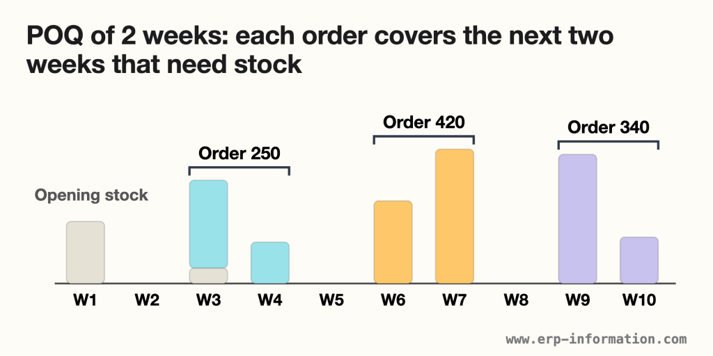
A purchased component has 150 units on hand, a one week lead time, an order cost of $90 and a holding cost of $0.40 per unit per week, charged on stock left at the end of each week. Gross requirements over ten weeks total 1,160 units, an average of 116 a week.
- EOQ = square root of (2 × 116 × 90 / 0.40) = 228.5 units
- POQ = 228.5 / 116 = 1.97, which rounds to 2 weeks
Net requirements equal gross requirements in every week except two: opening stock covers week 1 completely, and the 30 units it leaves cut week 3’s net requirement to 170.
| Wk | Gross | Receipt | Release | On hand |
|---|---|---|---|---|
| 1 | 120 | 0 | 0 | 30 |
| 2 | 0 | 0 | 250 | 30 |
| 3 | 200 | 250 | 0 | 80 |
| 4 | 80 | 0 | 0 | 0 |
| 5 | 0 | 0 | 420 | 0 |
| 6 | 160 | 420 | 0 | 260 |
| 7 | 260 | 0 | 0 | 0 |
| 8 | 0 | 0 | 340 | 0 |
| 9 | 250 | 340 | 0 | 90 |
| 10 | 90 | 0 | 0 | 0 |
Read it row by row. The first net requirement falls in week 3, so the first order covers weeks 3 and 4 (170 + 80 = 250) and is released in week 2 to allow for the lead time. Week 5 is empty, so the next cycle starts in week 6 and covers weeks 6 and 7 (420). Week 8 is empty again, so the last order covers weeks 9 and 10 (340).
The same requirements under six other rules
| Rule | Orders | Total cost | Above best |
|---|---|---|---|
| Wagner-Whitin (best possible) | 4 | $452.00 | 0% |
| Silver-Meal | 4 | $452.00 | 0% |
| POQ (2 weeks) | 3 | $466.00 | 3.1% |
| Part period balancing (textbook) | 3 | $466.00 | 3.1% |
| Least unit cost | 4 | $520.00 | 15.0% |
| Lot-for-lot | 6 | $564.00 | 24.8% |
| Fixed EOQ (228 units) | 5 | $746.80 | 65.2% |
Total cost is $90 per order plus $0.40 for every unit held at the end of a week. Every rule also carries the opening stock’s 30 units through weeks 1 and 2, which adds the same $24 to each.
POQ lost $14 in one place. Its fixed two-week window folded week 7’s 260 units into the week 6 order, and holding 260 units for a week costs 260 × $0.40 = $104, more than the $90 a separate order would have cost. The best plan orders weeks 6 and 7 separately, and $104 minus $90 is exactly the $14 gap. A fixed interval cannot see a large requirement landing at the end of its window.
The fixed EOQ did worst because 228-unit lots never lined up with the requirements: it carried stock almost every week and still had 138 units left after week 10.
How close does POQ get to the cheapest plan?
One example proves little, so we ran six rules over 24,000 randomly generated 24-week plans and compared each with the Wagner-Whitin plan: the exact minimum-cost plan for known demand, published by Harvey M. Wagner and Thomson M. Whitin in 1958.
| Rule | Steady | Variable | Lumpy |
|---|---|---|---|
| Silver-Meal | 1.1% | 1.9% | 2.7% |
| POQ | 0.9% | 8.9% | 7.3% |
| Part period balancing (textbook) | 8.6% | 10.2% | 9.7% |
| Least unit cost | 1.3% | 16.9% | 11.8% |
| Lot-for-lot | 62.1% | 75.2% | 33.5% |
| Fixed EOQ | 34.2% | 43.4% | 49.9% |
Each figure is the average cost above the cheapest possible plan. Steady demand has a standard deviation of 20% of its average, variable demand 60%, and lumpy demand has no requirement at all in 40% of weeks.
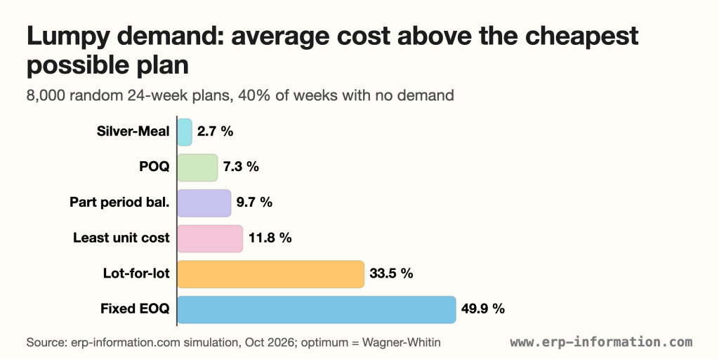
Three things stand out:
- On steady demand POQ is nearly perfect. It averaged 0.9% above the minimum and came within 5% of it in 99% of plans.
- On uneven demand it gives up 7% to 9%. It landed within 5% of the minimum in only 24% of variable plans and 46% of lumpy ones, because the interval is set from average demand and ignores the pattern inside each window.
- Silver-Meal averaged under 3% on every demand pattern and is no harder to work by hand: extend each order one period at a time while the average cost per period keeps falling. E. A. Silver and H. C. Meal published it in 1973. Being “dynamic” is no guarantee, though: part period balancing in its textbook form and least unit cost did worse than POQ on uneven demand. SAP’s version of part period balancing did better, as our part period balancing guide shows.
Lot-for-lot only did well where ordering is cheap. When one order costs less than about 1.1 times the cost of holding one period’s average demand for one period, POQ rounds to 1 and becomes lot-for-lot, so the two rules give the same plan.
How the test was run (9 October 2026): 2,000 plans for each of 3 demand patterns and 4 cost ratios, chosen so the EOQ covers 1, 2, 3 or 4 periods. Average demand 100 units a period, holding cost charged on ending stock, no opening stock, demand known for the whole 24 weeks. Steady demand was drawn from a normal distribution, variable demand from a gamma distribution, and lumpy demand from a gamma distribution with 40% of periods set to zero. Our code reproduces the EOQ and POQ plans in Gardner’s published worksheet, and its Wagner-Whitin solver matched a brute-force search on 300 small test cases. A second run with a different random seed moved no figure by more than 0.2 points. The test leaves out forecast error, capacity limits, quantity discounts and minimum order quantities, all of which add cost to every rule.
Disadvantages of Period Order Quantity
As an MRP rule, POQ has five real weaknesses:
- It is not the cheapest plan. On uneven demand it averaged 7% to 9% above the minimum in the test above, where Silver-Meal averaged under 3%.
- It is blind to what happens inside the window. The week 7 example shows the cost: a large requirement at the end of an interval gets carried when a separate order would be cheaper.
- The interval goes stale. It is computed from average demand and from cost figures. When demand, order cost or holding cost change, the POQ has to be recalculated, and nothing in the rule tells you when.
- It carries cycle stock. Each order holds up to POQ minus 1 periods of requirements. That is the price of fewer orders, and it grows with a longer interval.
- It makes component demand lumpier. In MRP, a parent item’s planned orders become its components’ gross requirements, so a two-week POQ on the parent drops two weeks of component demand into one week.
Two risks often listed for POQ belong to the purchasing sense, where a standard quantity arrives every period under a blanket order: deliveries that keep coming after usage falls, and stockouts when demand jumps late in the period. MRP-driven POQ avoids the first, because it only plans an order when there is a net requirement. It shares the second with every rule that plans from a forecast, which is what safety stock is for.
Lot Sizing Techniques

Period order quantity is one of several lot-sizing techniques. Each one answers the same question differently: how much should one order cover?
| Technique | How each order is sized |
|---|---|
| Lot-for-lot (L4L) | Exactly one period’s net requirement |
| Fixed order quantity (FOQ) | A set quantity, often a pack size or supplier minimum |
| Economic order quantity (EOQ) | A set quantity that balances order and holding cost for steady demand |
| Periods of supply (POS) | The net requirements of a number of periods the planner chooses |
| Period order quantity (POQ) | The net requirements of EOQ ÷ average demand periods |
| Least unit cost (LUC) | Adds periods while the cost per unit keeps falling |
| Least total cost (LTC) | Adds periods until holding cost comes closest to the order cost |
| Part period balancing (PPB) | The same balance test, published by J. J. DeMatteis in the IBM Systems Journal in 1968 |
| Silver-Meal | Adds periods while the cost per period keeps falling |
| Wagner-Whitin | Solves for the cheapest plan over the whole horizon |
POQ is periods of supply with the number of periods taken from the EOQ. In practice that means you calculate the POQ and enter it as the period in your system’s periods-of-supply setting. For the balance test in detail, see our part period balancing guide; for where lot sizing sits in the planning run, see material requirements planning.
Choosing the lot-sizing rule matters because it sets inventory levels, the number of orders and the load on capacity, and in MRP it also shapes the demand every component below the item sees.
How to set up POQ in an ERP system
In the four systems below, the length of the period is a setting you enter. Calculate the POQ with the formula, then put it in the field that matches. Checked against each vendor’s documentation on 9 October 2026:
- Oracle NetSuite: set the item’s supply lot sizing method to Periods of Supply. The type can be Interval, Weekly or Monthly; for Interval, the Period of Supply Increment takes a number from 1 to 90. NetSuite totals requirements from the first day an order is required and places the order on the first day of the period.
- Microsoft Dynamics 365 Business Central: use the Lot-for-Lot reordering policy with a Lot Accumulation Period. From the first planned supply, Business Central accumulates all supply needs in that period into one order, placed on the date of the first supply.
- Microsoft Dynamics 365 Supply Chain Management: use the Per period coverage code. The period starts with the item’s first demand, covers the length you define, and the next period starts with the next requirement, which is POQ’s behaviour exactly.
- SAP S/4HANA: use a period lot-sizing procedure. Periods can be days, weeks, months, posting periods or freely defined periods in a planning calendar, and the availability date defaults to the first requirement date in the period. SAP also offers optimum lot-sizing procedures, including part period balancing.
One difference matters in practice. NetSuite’s Interval type, Business Central and Dynamics 365 start the window at the first requirement, as textbook POQ does. SAP’s periods are fixed buckets (days, weeks, months or calendar periods), so the same requirements can be grouped differently from the textbook answer.
What is Economic Order Quantity?
Economic order quantity is the order size that minimises the combined cost of placing orders and holding stock when demand is steady. Larger orders mean fewer order costs but more stock on the shelf; the EOQ is the point where the two balance. It is one of the core techniques of inventory management, and holding cost here covers the inventory costs of keeping a unit in stock for a year.
The basic EOQ formula works when demand, order cost and holding cost stay constant, the whole order arrives at once, and there are no quantity discounts.
The formula for the calculation of Economic Order Quantity is Q = the square root of (2DS / H)
Note that the whole expression 2DS / H sits inside the square root. Writing it as the square root of 2DS, then divided by H, gives a different and incorrect answer.
Here,
- Q = Units of EOQ
- D = Demand in Units (Annual basis)
- S = Order Cost (per purchase)
- H = Holding Cost (per unit, per year)
With D = 48,000, S = $150 and H = $1.60, the formula gives the 3,000 units used in the POQ example above.
Click here for the Online Economic Order Quantity (EOQ) Calculator
Advantages of EOQ
- It gives the order size with the lowest combined order and holding cost under its assumptions.
- It is forgiving: total cost changes slowly near the EOQ, so an order somewhat larger or smaller costs little extra.
- It needs only three inputs, and it is the starting point for POQ.
- Paired with a reorder point, which decides when to order, it gives a complete replenishment policy for steady-demand items.
Disadvantages of EOQ
- It assumes demand is constant and known. Real demand moves, and order and holding costs change with freight rates, rents and interest rates.
- It assumes the whole order arrives at once. When stock builds up while it is produced, the production order quantity model below fits better.
- It ignores quantity discounts, which need a separate quantity discount model.
- On lumpy MRP demand, fixed lots leave remnants. In our test the fixed EOQ averaged 34% to 50% above the cheapest plan.
POQ vs EOQ: what is the difference?
POQ is derived from EOQ, but the two order in different ways. EOQ keeps the order quantity fixed and lets the timing float. POQ keeps the ordering interval fixed and lets the quantity match the actual demand in that interval, which is why it copes better with lumpy or uneven demand.
| EOQ (Economic Order Quantity) | POQ (Period Order Quantity) | |
|---|---|---|
| What stays fixed | The order quantity | The ordering interval (a set number of periods) |
| What varies | The time between orders | The order quantity |
| How it is set | Balances ordering cost against holding cost | Converts EOQ into a whole number of periods of demand |
| Best for | Steady, continuous demand | Lumpy or variable demand, common in MRP |
| Leftover stock | Can leave remnants when demand is uneven | Orders the exact demand for the interval, so little is left over |
| In our 24,000-plan test | 34% to 50% above the cheapest plan | 1% to 9% above the cheapest plan |
Production order quantity: the other POQ formula
If your question gives a daily production rate and a daily demand rate, it is asking for the production order quantity, not the period order quantity. Heizer, Render and Munson’s Operations Management uses this model when “inventory builds up over a period of time after an order is placed”, because units are produced and used at the same time.
Q* = square root of (2DS / (H × (1 − d/p)))
D is annual demand, S the setup cost, H the annual holding cost per unit, d the daily demand rate and p the daily production rate. Production must outpace demand, so p has to be larger than d. In the textbook’s own example, D = 1,000 units, S = $10, H = $0.50, p = 8 units a day and d = 4 units a day, which gives Q* = 282.8, or 283 units. The answer is a quantity of units, not a number of periods.
FAQs
The period order quantity is equal to what?
It equals the net requirements of the next N periods, where N is the EOQ divided by average demand per period, rounded to a whole number. Only the number of periods is fixed. The quantity changes with every order to match what those periods actually need.
Is period order quantity the same as a periodic review system?
No. A periodic review system counts stock at fixed intervals and orders enough to bring it up to a target level. Period order quantity is an MRP lot-sizing rule: it orders the exact net requirements of a set number of periods, and it plans no order at all when there is no net requirement.
What does a POQ of 1 mean?
Each order covers a single period, which is the same as lot-for-lot ordering. It happens when ordering is cheap relative to holding stock: when one order costs less than about 1.1 times the cost of holding one period of average demand for one period.
Does ASCM treat POQ as a fixed or a dynamic technique?
Both readings are used. ASCM’s CPIM Exam Content Manual version 8.0 grouped POQ with the dynamic techniques, and version 9.0, effective 1 June 2026, groups it with the fixed techniques alongside EOQ. The interval is fixed and the quantity varies.
How do I set up POQ in an ERP system?
Calculate the POQ, then enter it as the period length: Periods of Supply in Oracle NetSuite, a Lot Accumulation Period with the Lot-for-Lot policy in Business Central, the Per period coverage code in Dynamics 365 Supply Chain Management, or a period lot-sizing procedure in SAP S/4HANA.
Should you use POQ? A short decision guide
- Use POQ when demand is fairly steady, ordering is expensive enough that weekly orders waste money, and you or your supplier value a fixed ordering rhythm. On that kind of demand it averaged 0.9% above the best plan.
- Use Silver-Meal or an optimising rule instead when requirements are lumpy. On lumpy demand Silver-Meal averaged 2.7% above the best plan against POQ’s 7.3%. Test any other “dynamic” rule on your own data first: two of them did worse than POQ.
- Use lot-for-lot when POQ rounds to 1 period anyway, or for expensive items where holding cost dominates.
- Recalculate the interval whenever average demand, order cost or holding cost change, and check the answer by multiplying it back to the EOQ.
To size the inputs, see our gross requirements guide and the master production schedule that drives them.
How we researched this page
Updated 9 October 2026. Definitions and classifications come from ASCM’s CPIM exam content manuals, Gardner’s University of Houston MRP chapter and Heizer, Render and Munson’s course slides. ERP behaviour comes from each vendor’s current documentation, read on 9 October 2026. The MRP example and the 24,000-plan test are our own calculations, and the method is given above so you can repeat them.
References
- ASCM, CPIM Exam Content Manual, version 9.0, effective 1 June 2026, section VI.B.2.
- ASCM, CPIM Exam Content Manual, version 8.0, effective 1 June 2023, section V.B.2.
- Everette S. Gardner, Chapter 4, Material Requirements Planning, University of Houston, section 4.2 and Figure 4-2.
- Heizer, Render and Munson, Operations Management, chapter 12 slides, Pearson Education, 2017: EOQ robustness and the production order quantity model.
- H. M. Wagner and T. M. Whitin, Dynamic Version of the Economic Lot Size Model, Management Science 5(1), 89-96, 1958.
- J. J. DeMatteis, An economic lot-sizing technique, I: The part-period algorithm, IBM Systems Journal 7(1), 30-38, 1968.
- E. A. Silver and H. C. Meal, A heuristic for selecting lot size quantities for the case of a deterministic time-varying demand rate and discrete opportunities for replenishment, Production and Inventory Management 14(2), 64-74, 1973.
- Oracle, NetSuite: Setting Supply Planning Parameters.
- Microsoft Learn, Business Central: design details, planning parameters.
- Microsoft Learn, Dynamics 365 Supply Chain Management: coverage settings.
- SAP Help Portal, Period Lot-Sizing Procedures, SAP S/4HANA Material Requirements Planning, version 2025 FPS02.
Using Google Search? Add erp-information.com as a preferred source.